Integration of Geomappy into GeoPandas
import geopandas as gpd
import matplotlib.pyplot as plt
import geomappy as mp
import os
os.chdir("../../../")
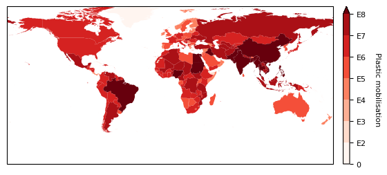
Loading data on river plastic mobilisation when flood events happen (Roebroek et al., 2021).
df1 = gpd.read_file("data/countries/plastic_mobilisation.shp")
df1.columns
Index(['featurecla', 'scalerank', 'LABELRANK', 'SOVEREIGNT', 'SOV_A3',
       'ADM0_DIF', 'LEVEL', 'TYPE', 'ADMIN', 'ADM0_A3',
       ...
       'NAME_ZH', 'e_1', 'e_10', 'e_20', 'e_50', 'e_100', 'e_200', 'e_500',
       'jump', 'geometry'],
      dtype='object', length=103)
Loading data on riverbank plastic observations in the Netherlands (Van Emmerik et al., 2020)
df2 = gpd.read_file("data/processed_data_SDN/df_locations.geojson")
df2.columns
Index(['Gebiedscode', 'river', 'x_maas', 'x_waal', 'geometry'], dtype='object')
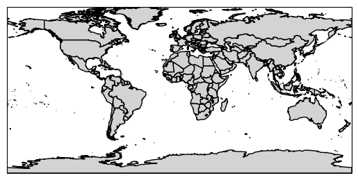
Outline on a world map
The first file covers the world, while the second file covers the Netherlands. Both have different projections. Geomappy allows to visualise it like this:
df1.plot_world()
df2.plot_world()
plt.show()


Plotting the data
The geomappy plotting functionality (plot_shapes) is directly
integrated into geopandas by loading geomappy. This results in the same
figure as seen before:
df1.plot_shapes()
plt.show()
df2.plot_shapes()
plt.show()

Again all plotting functionaly of plot_shapes is available. This is
shown here by reproducing the same map as in the tutorial on choropleth
continues shapes tutorial
im, cbar = df1.plot_shapes(
    values='e_10',
    cmap="Reds",
    bins=[0,100,1000,10000,100000,1000000, 10000000, 100000000]
)
cbar.ax.set_yticklabels([0, "E2", "E3", "E4", "E5", "E6", "E7", "E8"], fontsize=8)
cbar.set_label("Plastic mobilisation", labelpad=15, rotation=270, fontsize=8)
plt.show()